Exampville Destination Choice
In this notebook, we will walk through the estimation of a tour destination choice model for Exampville, an entirely fictional town built for the express purpose of demostrating the use of discrete choice modeling tools for transportation planning.
This example will assume the reader is familiar with the mathematical basics of destination choice modeling generally, and will focus on the technical aspects of estimating the parameters of a destination choice model in Python using Larch.
If you have not yet estimated parameters of a mode choice model or generated logsums from that model, you should go back and review those sections before you begin this one.
[1]:
import larch, numpy, pandas, os
from larch import P, X
Data Preparation
To begin, we will re-load the data files from our tour mode choice example.
[2]:
import larch.exampville

hh = pandas.read_csv( larch.exampville.files.hh )
pp = pandas.read_csv( larch.exampville.files.person )
tour = pandas.read_csv( larch.exampville.files.tour )
skims = larch.OMX( larch.exampville.files.skims, mode='r' )
We’ll also load an employment file. This file contains employment data by TAZ. The TAZ’s will be the choices in the destination choice model, and the employment data will allow us to characterize the number of opportunities in each TAZ.
[3]:
emp = pandas.read_csv(larch.exampville.files.employment, index_col='TAZ')
emp.info()
<class 'pandas.core.frame.DataFrame'>
Int64Index: 40 entries, 1 to 40
Data columns (total 3 columns):
NONRETAIL_EMP    40 non-null int64
RETAIL_EMP       40 non-null int64
TOTAL_EMP        40 non-null int64
dtypes: int64(3)
memory usage: 1.2 KB
We’ll also load the saved logsums from the mode choice estimation.
[4]:
logsums = pandas.read_pickle('/tmp/logsums.pkl.gz')
We’ll replicate the pre-processing used in the mode choice estimation, to merge the household and person characteristics into the tours data, add the index values for the home TAZ’s, filter to include only work tours, and merge with the level of service skims. (If this pre-processing was computationally expensive, it would probably have been better to save the results to disk and reload them as needed, but for this model these commands will run almost instantaneously.)
[5]:
co = tour.merge(hh, on='HHID').merge(pp, on=('HHID', 'PERSONID'))
co["HOMETAZi"] = co["HOMETAZ"] - 1
co["DTAZi"] = co["DTAZ"] - 1
co = co[co.TOURPURP == 1]
co.index.name = 'CASE_ID'
For this destination choice model, we’ll want to use the mode choice logsums we calculated previously, and we’ll use these values as data. The alternatives in the destinations model are much more regular than in the mode choice model – the utility function for each destination will have a common form – we’ll use idca format to make data management simpler. This format maintains a data array in three dimensions instead of two: cases, alternatives, and variables. We can still use a
pandas.DataFrame to hold this data, but we’ll use a MultiIndex for one of the typical dimensions.
We already have one idca format variable: the logsums we loaded above. For a destination choice model, we’ll often also want to use distance –specifically, the distance from the known origin zone to each possible destination zones. We can create a distance variable as an array, selecting for each case in the co data a row from the ‘AUTO_DIST’ array that matches the correct origin zone (by index number). Note that we first load the skim array into memory using [:] and then select the
rows, to overcome a technical limitation of the PyTables library (which underpins the open matrix format) that prevents us from reading the final array directly from the file on disk.
[6]:
distance = pandas.DataFrame(
    skims.AUTO_DIST[:][co["HOMETAZi"], :],
    index=co.index,
    columns=skims.TAZ_ID,
)
The distance and logsum arrays are both currently formatted as single variables stored in two-dimensional format (cases by alternatives) but to concatenate them together, we can use the unstack command to convert each into a one-dimensional array. We’ll also use the rename command to ensure that each one-dimensional array is named appropriately, so that when they are concatenate the result will include the names of the variables.
[7]:
ca = pandas.concat([
    distance.stack().rename("distance"),
    logsums.stack().rename("logsum"),
], axis=1)
Now we have our two variables in the correct format:
[8]:
ca.head()
[8]:
| distance | logsum | ||
|---|---|---|---|
| CASE_ID | TAZ_ID | ||
| 0 | 1 | 3.355488 | -1.022226 |
| 2 | 4.133484 | -0.957339 | |
| 3 | 7.915948 | -2.826200 | |
| 4 | 3.856728 | -1.218908 | |
| 5 | 3.345056 | -1.185637 |
We’ll also need to join employment data to the ca DataFrame. This data has unique values only by alternative and not by caseid, so there are only 40 unique rows.
[9]:
emp.info()
<class 'pandas.core.frame.DataFrame'>
Int64Index: 40 entries, 1 to 40
Data columns (total 3 columns):
NONRETAIL_EMP    40 non-null int64
RETAIL_EMP       40 non-null int64
TOTAL_EMP        40 non-null int64
dtypes: int64(3)
memory usage: 1.2 KB
But to make this work with the computational arrays required for Larch, we’ll need to join this to the other idca data, like this:
[10]:
ca = ca.join(emp, on='TAZ_ID')
We can also extract an ‘Area Type’ variable from the skims, and attach that as well:
[11]:
area_type = pandas.Series(
    skims.TAZ_AREA_TYPE[:],
    index=skims.TAZ_ID[:],
    name ='TAZ_AREA_TYPE',
).astype('category')
[12]:
ca = ca.join(area_type, on='TAZ_ID')
Then we bundle the raw data into the larch.DataFrames structure, as we did for estimation, and attach this structure to the model as its dataservice.
[13]:
dfs = larch.DataFrames(
    co=co,
    ca=ca,
    alt_codes=skims.TAZ_ID,
    alt_names=['TAZ{i}' for i in skims.TAZ_ID],
    ch_name='DTAZ',
    av=True,
)
[14]:
dfs.info(1)
larch.DataFrames:  (not computation-ready)
  n_cases: 4952
  n_alts: 40
  data_ca:
    - distance
    - logsum
    - NONRETAIL_EMP
    - RETAIL_EMP
    - TOTAL_EMP
    - TAZ_AREA_TYPE
  data_co:
    - TOURID
    - HHID
    - PERSONID
    - DTAZ
    - TOURMODE
    - TOURPURP
    - X
    - Y
    - INCOME
    - geometry
    - HOMETAZ
    - HHSIZE
    - HHIDX
    - AGE
    - WORKS
    - N_WORK_TOURS
    - N_OTHER_TOURS
    - N_TOURS
    - HOMETAZi
    - DTAZi
  data_av: <populated>
  data_ch: DTAZ
Model Definition
[15]:
m = larch.Model(dataservice=dfs)
Destination choice models are premised on the theory that each trip or tour has a particular destination to which it is attracted, and each travel zone represents not one individual alternative, but rather a number of similar alternatives grouped together. Thus the utility function in a destination choice model typically is comprised of two components: a qualitative component (i.e., how good are the alternatives in a zone) and a quantitative component (i.e., how many discrete alternatives are in a zone). The mathematical form of the utility function for the zone is
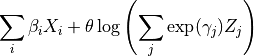
The quantitative component of this utility function is written for Larch in a linear-in-parameters format similarly to that for the typical utility function, but assigned to the quantity_ca attribute instead of utility_ca. Also, the exponentiation of the  parameters is implied by using
 quantity_ca. Note that the quantitative term is in theory always applied only to the alternatives themselves and not alone to attributes of the decision maker, so the quantity_co
attribute is not implemented and cannot be used.
[16]:
m.quantity_ca = (
        + P.EmpRetail_HighInc * X('RETAIL_EMP * (INCOME>50000)')
        + P.EmpNonRetail_HighInc * X('NONRETAIL_EMP') * X("INCOME>50000")
        + P.EmpRetail_LowInc * X('RETAIL_EMP') * X("INCOME<=50000")
        + P.EmpNonRetail_LowInc * X('NONRETAIL_EMP') * X("INCOME<=50000")
)
The parameter  is a coefficient on the entire log-of-quantity term, and can be defined by assigning a parameter name to the
 quantity_scale attribute.
[17]:
m.quantity_scale = P.Theta
The qualitative component of utility can be given in the same manner as any other discrete choice model in Larch.
[18]:
m.utility_ca = (
    + P.logsum * X.logsum
    + P.distance * X.distance
)
For this structure, we know the model will be overspecified if the parameter in the quantitative portion of utility are all estimated, in a manner similar to the overspecification if alternative specific constants are all estimated. To prevent this problem, we can lock parameters to particular values as needed using the lock_values method.
[19]:
m.lock_values(
    EmpRetail_HighInc=0,
    EmpRetail_LowInc=0,
)
Then let’s prepare this data for estimation. Even though the data is already in memory, the load_data method is used to pre-process the data, extracting the required values, pre-computing the values of fixed expressions, and assembling the results into contiguous arrays suitable for computing the log likelihood values efficiently.
[20]:
m.load_data()
req_data does not request {choice_ca,choice_co,choice_co_code} but choice is set and being provided
req_data does not request avail_ca or avail_co but it is set and being provided
Model Estimation
[21]:
m.maximize_loglike()
Iteration 005 [Converged]
LL = -16366.830847931089
| value | initvalue | nullvalue | minimum | maximum | holdfast | note | best | |
|---|---|---|---|---|---|---|---|---|
| EmpNonRetail_HighInc | 0.903947 | 0.0 | 0.0 | -inf | inf | 0 | 0.903947 | |
| EmpNonRetail_LowInc | -0.997606 | 0.0 | 0.0 | -inf | inf | 0 | -0.997606 | |
| EmpRetail_HighInc | 0.000000 | 0.0 | 0.0 | 0.000 | 0.0 | 1 | 0.000000 | |
| EmpRetail_LowInc | 0.000000 | 0.0 | 0.0 | 0.000 | 0.0 | 1 | 0.000000 | |
| Theta | 0.728573 | 1.0 | 1.0 | 0.001 | 1.0 | 0 | 0.728573 | |
| distance | 0.006269 | 0.0 | 0.0 | -inf | inf | 0 | 0.006269 | |
| logsum | 1.200129 | 0.0 | 0.0 | -inf | inf | 0 | 1.200129 |
[21]:
| key | value | ||||||||||||||||
|---|---|---|---|---|---|---|---|---|---|---|---|---|---|---|---|---|---|
| loglike | -16366.83084793109 | ||||||||||||||||
| x |
| ||||||||||||||||
| tolerance | 2.528376923579841e-07 | ||||||||||||||||
| steps | array([1., 1., 1., 1., 1.]) | ||||||||||||||||
| message | 'Optimization terminated successfully.' | ||||||||||||||||
| elapsed_time | 0:00:00.184758 | ||||||||||||||||
| method | 'bhhh' | ||||||||||||||||
| n_cases | 4952 | ||||||||||||||||
| iteration_number | 5 | ||||||||||||||||
| logloss | 3.3050950823770378 |
After we find the best fitting parameters, we can compute some variance-covariance statistics, incuding standard errors of the estimates and t statistics, using calculate_parameter_covariance.
[22]:
m.calculate_parameter_covariance()
Then we can review the results in a variety of report tables.
[23]:
m.parameter_summary()
[23]:
| Parameter | Value | Std Err | t Stat | Null Value |
|---|---|---|---|---|
| EmpNonRetail_HighInc | 0.9039 | 0.279 | 3.24 | 0.0 |
| EmpNonRetail_LowInc | -0.9976 | 0.0961 | -10.39 | 0.0 |
| EmpRetail_HighInc | 0 | fixed value | ||
| EmpRetail_LowInc | 0 | fixed value | ||
| Theta | 0.7286 | 0.0181 | -14.98 | 1.0 |
| distance | 0.006269 | 0.0156 | 0.40 | 0.0 |
| logsum | 1.2 | 0.0483 | 24.86 | 0.0 |
[24]:
m.estimation_statistics()
[24]:
| Statistic | Aggregate | Per Case |
|---|---|---|
| Number of Cases | 4952 | |
| Log Likelihood at Convergence | -16366.83 | -3.31 |
| Log Likelihood at Null Parameters | -18362.98 | -3.71 |
| Rho Squared w.r.t. Null Parameters | 0.109 | |
[25]:
m.utility_functions()
[25]:
| + P.logsum * X.logsum + P.distance * X.distance + P.Theta * log( + exp(P.EmpRetail_HighInc) * X('RETAIL_EMP * (INCOME>50000)') + exp(P.EmpNonRetail_HighInc) * X('NONRETAIL_EMP*(INCOME>50000)') + exp(P.EmpRetail_LowInc) * X('RETAIL_EMP*(INCOME<=50000)') + exp(P.EmpNonRetail_LowInc) * X('NONRETAIL_EMP*(INCOME<=50000)') ) |
Model Visualization
For destination choice and similar type models, it might be beneficial to review the observed and modeled choices, and the relative distribution of these choices across different factors. For example, we would probably want to see the distribution of travel distance. The Model object includes a built-in method to create this kind of visualization.
[26]:
m.distribution_on_idca_variable('distance')
[26]:
[27]:
m.distribution_on_idca_variable(
    m.dataservice.data_ca.TAZ_AREA_TYPE
)
[27]:
The distribution_on_idca_variable has a variety of options, for example to control the number and range of the histogram bins:
[28]:
m.distribution_on_idca_variable('distance', bins=40, range=(0,10))
[28]:
Alternatively, the histogram style can be swapped out for a smoothed kernel density function, by setting the style argument to 'kde'.
[29]:
m.distribution_on_idca_variable(
    'distance',
    style='kde',
    range=(0,13),
)
[29]:
Subsets of the observations can be pulled out, to observe the distribution conditional on other idco factors, like income.
[30]:
m.distribution_on_idca_variable(
    'distance',
    subselector='INCOME<10000',
)
[30]:
It is also possible to customize some cosmetic parts of the generated figure, for example attaching a title or giving a more detailed and well formatted label for the x-axis.
[31]:
m.distribution_on_idca_variable(
    'distance',
    xlabel="Distance (miles)",
    bins=26,
    subselector='INCOME<10000',
    range=(0,13),
    header='Destination Distance, Very Low Income (<$10k) Households',
)
Alternatively, a matplotlib.Axes instance can be passed to the distribution_on_idca_variable function as the ax argument, and the figure will be drawn there. This allows full customizability of the rest of the figure using the usual matplotlib features.
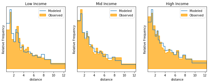
[32]:
from matplotlib import pyplot as plt
fig, axes = plt.subplots(1,3, figsize=(12,4))

income_categories = {
    'Low Income': 'INCOME<10000',
    'Mid Income': '(10000<=INCOME) & (INCOME<50000)',
    'High Income': 'INCOME>=50000',
}

for ax, (inc_title, inc) in zip(axes, income_categories.items()):
    m.distribution_on_idca_variable(
        'distance',
        subselector=inc,
        ax=ax,
        range=(0,13),
    )
    ax.set_title(inc_title)
Save and Report Model
If we are satisified with this model, or if we just want to record it as part of our workflow while exploring different model structures, we can write the model out to a report. To do so, we can instantiatie a larch.Reporter object.
[33]:
report = larch.Reporter(title=m.title)
Then, we can push section headings and report pieces into the report using the “<<” operator.
[34]:
report << '# Parameter Summary' << m.parameter_summary()
[34]:
[35]:
report << "# Estimation Statistics" << m.estimation_statistics()
[35]:
[36]:
report << "# Utility Functions" << m.utility_functions()
[36]:
Utility Functions
| + P.logsum * X.logsum + P.distance * X.distance + P.Theta * log( + exp(P.EmpRetail_HighInc) * X('RETAIL_EMP * (INCOME>50000)') + exp(P.EmpNonRetail_HighInc) * X('NONRETAIL_EMP*(INCOME>50000)') + exp(P.EmpRetail_LowInc) * X('RETAIL_EMP*(INCOME<=50000)') + exp(P.EmpNonRetail_LowInc) * X('NONRETAIL_EMP*(INCOME<=50000)') ) |
Once we have assembled the report, we can save the file to disk as an HTML report containing the content previously assembled. Attaching the model itself to the report as metadata can be done within the save method, which will allow us to directly reload the same model again later.
[37]:
report.save(
    '/tmp/exampville_destination_choice.html',
    overwrite=True,
    metadata=m,
)
[37]:
'/tmp/exampville_destination_choice.html'