Using Static Mapping

import transportation_tutorials as tt
import geopandas as gpd
import pandas as pd
import matplotlib.pyplot as plt
import numpy as np
from shapely.geometry import Polygon, Point

Questions

1. Generate a population density map of Miami-Dade County, at the MAZ resolution level for SERPM 8. (Hint: Clip the maximum population density at 40,000 persons per square mile.)

Data

To answer the question, use the following files:

maz = gpd.read_file(tt.data('SERPM8-MAZSHAPE'))
maz.head()

	OBJECTID	MAZ	SHAPE_LENG	SHAPE_AREA	ACRES	POINT_X	POINT_Y	geometry
0	1	5347	8589.393674	3.111034e+06	71	953130	724165	POLYGON ((953970.4660769962 723936.0810402408,...
1	2	5348	11974.067469	7.628753e+06	175	907018	634551	POLYGON ((908505.2801046632 635081.7738410756,...
2	3	5349	9446.131753	4.007041e+06	92	923725	707062	POLYGON ((922736.6374686621 708387.6918614879,...
3	4	5350	21773.153739	2.487397e+07	571	908988	713484	POLYGON ((908334.2374677472 715692.2628822401,...
4	5	5351	17882.701416	1.963139e+07	451	909221	717493	POLYGON ((911883.0187559947 719309.3261861578,...

maz_data = pd.read_csv(tt.data('SERPM8-MAZDATA', '*.csv'))
maz_data.head()

	mgra	TAZ	HH	POP	emp_self	emp_ag	emp_const_non_bldg_prod	emp_const_non_bldg_office	emp_utilities_prod	emp_utilities_office	...	EmpDenBin	DuDenBin	POINT_X	POINT_Y	ACRES	HotelRoomTotal	mall_flag	beachAcres	geoSRate	geoSRateNm
0	1	2901	43	169	0	0	0	0	0	0	...	1	1	841743	586817	510	0	0	0	1	1
1	2	2902	9	21	0	1	1006	0	8	0	...	1	1	855391	585688	5678	0	0	0	1	1
2	3	2903	403	1389	0	0	6	0	0	0	...	1	1	858417	549492	85	0	0	0	1	1
3	4	2903	477	1659	0	0	3	0	0	0	...	1	1	858468	552269	103	0	0	0	1	1
4	5	2903	374	1389	0	0	11	0	0	0	...	1	1	859899	552161	72	0	0	0	1	1

5 rows × 76 columns

fl_county = gpd.read_file(tt.data('FL-COUNTY-SHAPE'))
fl_county.head()

	OBJECTID	DEPCODE	COUNTY	COUNTYNAME	DATESTAMP	ShapeSTAre	ShapeSTLen	geometry
0	1	21	041	GILCHRIST	2000-05-16T00:00:00.000Z	9.908353e+09	4.873000e+05	POLYGON ((-82.65813600527831 29.83028106592836...
1	2	54	107	PUTNAM	2000-05-16T00:00:00.000Z	2.305869e+10	7.629677e+05	POLYGON ((-81.58084263191225 29.83955869988373...
2	3	62	123	TAYLOR	2000-05-16T00:00:00.000Z	2.891747e+10	8.772527e+05	(POLYGON ((-83.73036687278116 30.3035764144186...
3	4	46	091	OKALOOSA	2000-05-16T00:00:00.000Z	2.562159e+10	1.087058e+06	(POLYGON ((-86.39159408384468 30.6497039172779...
4	5	7	013	CALHOUN	2000-05-16T00:00:00.000Z	1.604809e+10	6.313440e+05	POLYGON ((-84.93265667941331 30.60636534524649...

Solution

We can begin by extracting just Miami-Dade county from the counties shapefile. As noted, the name is recorded in this file as just “DADE”, so we can use that to get the correct county.

md_county = fl_county.query("COUNTYNAME == 'DADE'")

The county shapefile uses a different crs, so we’ll need to make them aligned before doing a join.

md_county = md_county.to_crs({'init': 'epsg:2236', 'no_defs': True})

md_polygon = md_county.iloc[0].geometry

Next, we can select the MAZ centroids that are within the Miami-Dade polygon.

md_maz = maz[maz.centroid.within(md_polygon)]

Then we merge maz_data dataframe with spatially joined md_maz to pull in the required population information.

md_maz_info = md_maz.merge(maz_data.astype(float)[['mgra', 'POP']], how = 'left', left_on = 'MAZ', right_on = 'mgra')

md_maz_info.head()

	OBJECTID	MAZ	SHAPE_LENG	SHAPE_AREA	ACRES	POINT_X	POINT_Y	geometry	mgra	POP
0	6678	1	22430.293060	2.220769e+07	510	841744	586819	POLYGON ((843052.3509714119 590418.30837816, 8...	1.0	169.0
1	6679	2	77075.035787	2.480557e+08	5695	855391	585705	POLYGON ((872650.4321950786 590666.4279606566,...	2.0	21.0
2	6680	3	8681.166565	3.704251e+06	85	858417	549492	POLYGON ((859334.5900604129 549311.0687424093,...	3.0	1389.0
3	6681	4	8629.955860	4.492026e+06	103	858468	552269	POLYGON ((859424.1906029955 553546.9969503209,...	4.0	1659.0
4	6682	5	8022.697944	3.140387e+06	72	859899	552161	POLYGON ((860482.4981976636 553546.9001657367,...	5.0	1389.0

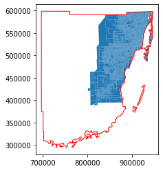
We can review a map of the selected MAZ’s and the Miami-Dade County borders. Note that the MAZ’s don’t actually cover the whole county, as the south and west areas of the county are undeveloped swampland.

ax = md_maz_info.plot()
md_county.plot(ax=ax, color='none', edgecolor='red');

Because the unit of measure in EPSG:2236 is approximately a foot, the area property of the md_maz_info GeoDataFrame gives the area in square feet. To express population density in persons per square mile, we need to multiply by 5280 (feet per mile) squared.

md_maz_info["Population Density"] = md_maz_info.POP / md_maz_info.area * 5280**2

A first attempt at drawing a population density choropleth shows something is wrong; the entire county is displayed as nearly zero.

fig, ax = plt.subplots(figsize=(12,9))
ax.axis('off') # don't show axis
ax.set_title("Population Density", fontweight='bold', fontsize=16)
ax = md_maz_info.plot(ax=ax, column="Population Density", legend=True)

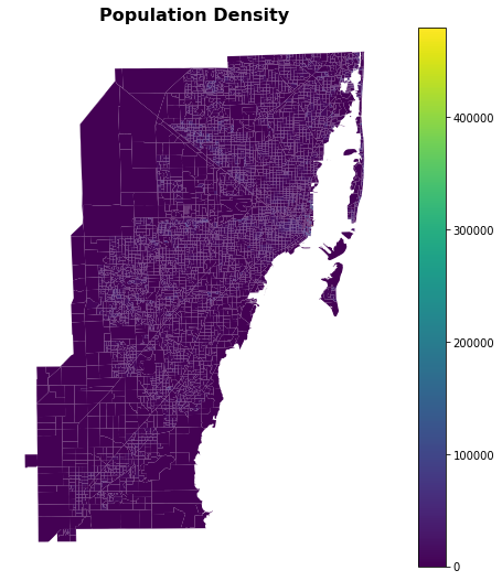
The problem is identifiable in the legend: the scale goes up to nearly half a million people per square mile, which is an enormous value, and generally not achievable unless a zone is basically just skyscrapers. This does apply to a handful of MAZ’s in downtown Miami, but the density everywhere else is so much lower that this map is meaningless.

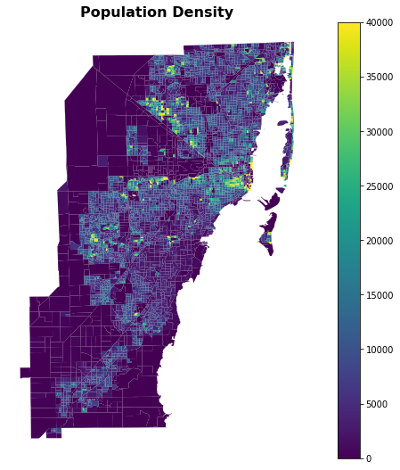
We can create a more meaningful map by clipping the top of the range to a more reasonable value, say only 40,000 people per square mile.

fig, ax = plt.subplots(figsize=(12,9))
ax.axis('off') # don't show axis
ax.set_title("Population Density", fontweight='bold', fontsize=16)
ax = md_maz_info.plot(ax=ax, column=np.clip(md_maz_info["Population Density"], 0, 40_000), legend=True)