[1]:
import transportation_tutorials as tt
Manipulating Geographic Data
A shapefile is a data format that is actually a set of files containing geospatial information. All of the related files have the same filename (except for the file extension) and must reside in the same directory. Generally, there will be files with the shp extension containing geographic data, the dbf extension containing tabular data, and a few others. The files can be read into python as a group and manipulated using the
GeoPandas package.
[2]:
import geopandas as gpd
Loading a Shapefile
Let’s load the SERPM8 TAZ shapefile. This shapefile (actually a set of files) is included in the data of the tuturials package and can be accessed as shown. Loading a shapefile into Python using geopandas is a simple task using the read_file function.
[3]:
shapefile_filename = tt.data('SERPM8-TAZSHAPE')
taz = gpd.read_file(shapefile_filename)
This will load the shapefile into a GeoDataFrame object, which is similar to a pandas DataFrame, but with a special geometry column that contains, as you might guess, geometric shape data contained in the shp part of the shapefile. It also includes all the other various tabular data contained in the dbf part of the shapefile. We can inspect the first few lines of the GeoDataFrame to see the contents, just like a regular DataFrame:
[4]:
taz.head()
[4]:
| OBJECTID | TAZ_REG | TAZ_OLD05 | TAZ_MPO | COUNTY | CENSUSTAZ | TAZ_BF | FIX | AREA | F_NETAREA | CBD | HM_ROOMS | Shape_Leng | Shape_Area | geometry | |
|---|---|---|---|---|---|---|---|---|---|---|---|---|---|---|---|
| 0 | 1 | 1122.0 | 1122 | 1122 | 1.0 | None | 0 | 0 | 4442490.0 | 0.8153 | 0 | 0 | 10592.846522 | 4.442490e+06 | POLYGON ((936374.6744969971 959539.5675094873,... |
| 1 | 2 | 17.0 | 17 | 17 | 1.0 | None | 0 | 0 | 15689400.0 | 0.8571 | 0 | 0 | 17396.297932 | 1.568938e+07 | POLYGON ((942254.5000076629 952920.9373740703,... |
| 2 | 3 | 1123.0 | 1123 | 1123 | 1.0 | None | 0 | 0 | 17396100.0 | 0.8663 | 0 | 0 | 23585.421941 | 1.739613e+07 | POLYGON ((940953.5610084943 952985.0688074902,... |
| 3 | 4 | 1120.0 | 1120 | 1120 | 1.0 | None | 0 | 0 | 1303420.0 | 0.8536 | 0 | 0 | 7202.864864 | 1.303422e+06 | POLYGON ((953118.9999321625 951985.3749407381,... |
| 4 | 5 | 1121.0 | 1121 | 1121 | 1.0 | None | 0 | 0 | 31477500.0 | 0.8787 | 0 | 0 | 24940.959492 | 3.147748e+07 | POLYGON ((934328.2825924121 951600.5853559896,... |
Because this is the TAZ shapefile, we expect that the geometry column includes a set of Polygon values, as we can observe in the first few rows. We can also easily check how many zones are included in the file by checking the length of the GeoDataFrame.
[5]:
len(taz)
[5]:
4236
Displaying the shapefile in a jupyter notebook can be accomplished by calling the plot method of the GeoDataFrame.
[6]:
ax = taz.plot()
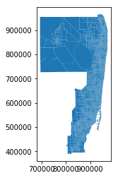
Coordinate Reference Systems
You might notice that the axis labels don’t show latitude and longitude. That’s because the TAZ file uses a different coordinate reference system (crs) for map projection. We can find what crs is being used by accessing the crs attribute.
[7]:
taz.crs
[7]:
{'init': 'epsg:2236'}
Drop that code into Google and you’ll find that it’s a special coordinate system for mapping and engineering in eastern Florida, which for this application may be perfectly reasonable. However, suppose we want to generate maps using plain old latitude and longitude. We can convert between CRS systems easily, like this:
[8]:
taz1 = taz.to_crs(epsg=4326)
[9]:
ax = taz1.plot()
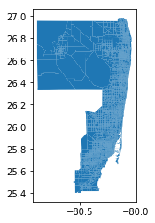
The map projection generated here is subtly different from the previous one. If you look carefully, you’ll note the shape of the second map is a bit wider than first. This distortion is a natural part of the mapping projection, using plain latitude and longitude, as one degree of longitude is a different distance than one degree of latitude. In Florida, the difference is relatively small, but it grows as you move north.
Selecting by Geography
The SERPM8 region is quite large. Let’s suppose we only want to study a small portion of this region. Since we are working with Jupyter notebooks, we’ll select an area to study around Jupiter, Florida.
Selection by Rectangular Envelope
We can explicitly define some bounds for our study area:
[10]:
xmin = 905712.145924
ymin = 905343.94408855
xmax = 983346.68922847
ymax = 981695.93140023
Then, to select only the TAZ’s that are (at least partially) contained in the study area, we can use the cx indexer on GeoDataFrames. This indexer works similarly to the loc and iloc indexers on regular DataFrames, but selects not based on labels or tabular position, but instead selects based on geographic position.
[11]:
taz_jupiter = taz.cx[xmin:xmax, ymin:ymax]
The result of the selection is another GeoDataFrame, just as slicing using the locand iloc indexers on regular DataFrames creates a new DataFrame. Thus, we can review how many TAZ’s are in the selection in the same manner as we checked the number of TAZ’s in the original shapefile.
[12]:
len(taz_jupiter)
[12]:
220
And we can plot a map of the selected area, just as we did with the original data. Here, we’ll draw the borders of the TAZ’s in white for better contrast.
[13]:
ax = taz_jupiter.plot(edgecolor='w')
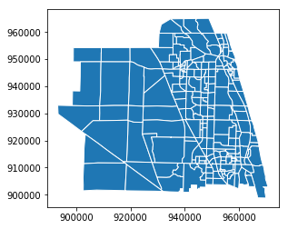
Because Jupiter is in the northwest corner of the SERPM region, only the south and west boundaries of the study area are relevant in the selection definition. Convenietly, just like other DataFrame indexers, the cx indexer allows for one-sided slices.
[14]:
taz_jupiter2 = taz.cx[xmin:, ymin:]
taz_jupiter2.equals(taz_jupiter)
[14]:
True
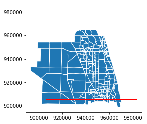
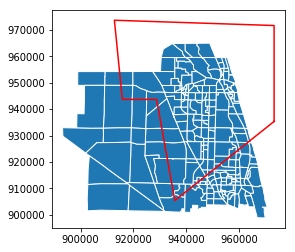
One important note regarding the cx indexer is that it will select all features that are contained fully or partially in the selection area. To illustrate, we can construct a GeoDataFrame consisting of the study area box, and draw it on a map of the selected zones.
[15]:
from shapely.geometry import box
study_area = gpd.GeoDataFrame(geometry=[box(xmin, ymin, xmax, ymax)], crs={'init': 'epsg:2236'})
ax = taz_jupiter.plot(edgecolor='w')
transparent = (0,0,0,0)
ax = study_area.plot(ax=ax, edgecolor='red', facecolor=transparent)
Selection by Polygon
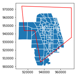
If the study area is not neatly defined by a rectangle but instead by some defined irregular polygon, it is still possible to filter the GeoDataFrame, but slightly more complicated. We’ll demonstrate by first constructing an irregular polygon.
[16]:
from shapely.geometry import Polygon
irregular_polygon = Polygon([
    (973346, 935343),
    (973346, 971695),
    (912812, 973695),
    (915812, 943695),
    (928812, 943695),
    (935712, 905343),
])
ax = taz_jupiter.plot(edgecolor='w')
lines = ax.plot(*irregular_polygon.exterior.xy, color='r')
To indentify those TAZ polygons that touch the polygon, we can use the intersects method of GeoDataFrames.
[17]:
taz_jupiter.intersects(irregular_polygon)
[17]:
0        True
1        True
2        True
3        True
4        True
5        True
6        True
7        True
8        True
9        True
10       True
11       True
12       True
13       True
14       True
15       True
16       True
17       True
18       True
19       True
20       True
21       True
22       True
23       True
24       True
25       True
26       True
27       True
28       True
29       True
        ...
755     False
756     False
1455    False
1462     True
1463     True
1464     True
1465     True
1466     True
1467    False
1468    False
1469    False
1491    False
1497     True
1498     True
1499     True
1500    False
1501    False
1631     True
1632    False
1635    False
1636     True
1637     True
1638     True
1639     True
1640     True
1641     True
1642     True
1643     True
1644     True
1645     True
Length: 220, dtype: bool
This gives us a series that matches the GeoDataFrame, and identifies whether each row’s geometry intersects the the polygon. We can use that to filter the rows, to retain only those TAZ’s of interest.
[18]:
taz_jupiter_irregular = taz_jupiter[taz_jupiter.intersects(irregular_polygon)]
[19]:
len(taz_jupiter_irregular)
[19]:
146
This gives us a new GeoDataFrame that is potentially just a filtered view of the original, which can potentially lead to problems later (see here). To ensure we have a bonafide new GeoDataFrame, we can make sure it is a copy.
[20]:
taz_jupiter_irregular = taz_jupiter_irregular.copy()
[21]:
ax = taz_jupiter_irregular.plot(edgecolor='w')
lines = ax.plot(*irregular_polygon.exterior.xy, color='r')
You may note, as with the rectangular selection, we still select any zone that has any part of the zone inside the polygon.
Clipping by Geography
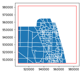
If instead we want to actually clip the geographic data at the study area frame, we can use the overlay function to get the intersection of the TAZ’s and the study area.
[22]:
taz_jupiter_clip = gpd.overlay(taz, study_area, how='intersection')
By taking the intersection, we discard portions of the zone shapes that are outside the study area, as is illustrated when we map the results with the study area box.
[23]:
ax = taz_jupiter_clip.plot(edgecolor='w')
transparent = (0,0,0,0)
ax = study_area.plot(ax=ax, edgecolor='red', facecolor=transparent)
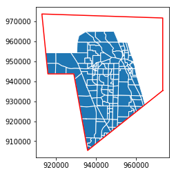
Alternatively, if we have a polygon, we can use intersection to trim the GeoDataFrame geometry to only the overlapping areas.
[24]:
taz_jupiter_irregular.geometry = taz_jupiter_irregular.intersection(irregular_polygon)
[25]:
ax = taz_jupiter_irregular.plot(edgecolor='w')
transparent = (0,0,0,0)
lines = ax.plot(*irregular_polygon.exterior.xy, color='r')
An important feature to consider if using this method is that the operation does not actually change the set of rows or any other data included in the GeoDataFrame. If, for example, we apply it to the set of TAZ’s from the square clipped region, we can get a map that looks identical, but the GeoDataFrame will still retain all the data rows from the previous version, just with some geometry values set as empty.
[26]:
taz_jupiter_clip.geometry = taz_jupiter_clip.intersection(irregular_polygon)

ax = taz_jupiter_clip.plot(edgecolor='w')
transparent = (0,0,0,0)
lines = ax.plot(*irregular_polygon.exterior.xy, color='r')

[27]:
len(taz_jupiter_irregular), len(taz_jupiter_clip)
[27]:
(146, 220)
[28]:
sum(taz_jupiter_clip.geometry.area == 0)
[28]:
74
Joining by Geography
A common task in geographic analysis is joining two sets of geographic data together. We actually did a simple version of this just above, when we joined the TAZ data with the study area, although the study area had only a single polygon and no other associated data, so the results are not particularly inspiring.
As a more sophisticated example, let’s consider the micro-area zone (MAZ) system from SERPM8. The MAZ are smaller zones nested inside TAZ’s, used to provide a higher resolution of data, particularly for transit travel. Using the TAZ system is sometimes too coarse for this purpose, as it may be convenient to walk to a bus stop located on a TAZ boundary only for some parts of the zone, while the walking from the far side of the same TAZ to the bus stop might be unreasonably far.
Like the TAZ system, the MAZ system for SERPM8 is given by a shape file, and is included in the tutorial data, so we can load it in the same way.
[29]:
mazshape_filename = tt.data('SERPM8-MAZSHAPE')
maz = gpd.read_file(mazshape_filename)
[30]:
len(maz)
[30]:
12022
[31]:
maz.head()
[31]:
| OBJECTID | MAZ | SHAPE_LENG | SHAPE_AREA | ACRES | POINT_X | POINT_Y | geometry | |
|---|---|---|---|---|---|---|---|---|
| 0 | 1 | 5347 | 8589.393674 | 3.111034e+06 | 71 | 953130 | 724165 | POLYGON ((953970.4660769962 723936.0810402408,... |
| 1 | 2 | 5348 | 11974.067469 | 7.628753e+06 | 175 | 907018 | 634551 | POLYGON ((908505.2801046632 635081.7738410756,... |
| 2 | 3 | 5349 | 9446.131753 | 4.007041e+06 | 92 | 923725 | 707062 | POLYGON ((922736.6374686621 708387.6918614879,... |
| 3 | 4 | 5350 | 21773.153739 | 2.487397e+07 | 571 | 908988 | 713484 | POLYGON ((908334.2374677472 715692.2628822401,... |
| 4 | 5 | 5351 | 17882.701416 | 1.963139e+07 | 451 | 909221 | 717493 | POLYGON ((911883.0187559947 719309.3261861578,... |
[ ]:
We can select only MAZ’s in the study area in the same manner as we did for TAZ’s.
[32]:
maz_jupiter = maz.cx[xmin:xmax, ymin:ymax]
[33]:
len(maz_jupiter)
[33]:
361
To create a joined GeoDataFrame, we can use the same `overlay <http://geopandas.org/reference/geopandas.overlay.html>`__ function we used to clip the TAZ’s, although we will intersect the TAZ and MAZ geometries.
[34]:
maz_taz = gpd.overlay(maz_jupiter, taz_jupiter, how='intersection')
The joined GeoDataFrame has all the columns from both the MAZ and TAZ source data. In cases where both source tables have an identically named column (for example, “OBJECTID”) then both columns are retained, and they are labeled with “_1” and “_2” suffixes.
[35]:
maz_taz.head()
[35]:
| OBJECTID_1 | MAZ | SHAPE_LENG | SHAPE_AREA | ACRES | POINT_X | POINT_Y | OBJECTID_2 | TAZ_REG | TAZ_OLD05 | ... | CENSUSTAZ | TAZ_BF | FIX | AREA | F_NETAREA | CBD | HM_ROOMS | Shape_Leng | Shape_Area | geometry | |
|---|---|---|---|---|---|---|---|---|---|---|---|---|---|---|---|---|---|---|---|---|---|
| 0 | 2389 | 7736 | 10592.846522 | 4.442490e+06 | 102 | 936259 | 957308 | 1 | 1122.0 | 1122 | ... | None | 0 | 0 | 4442490.0 | 0.8153 | 0 | 0 | 10592.846522 | 4.442490e+06 | POLYGON ((936374.6744969971 959539.5675094873,... |
| 1 | 2390 | 7737 | 17396.297932 | 1.568938e+07 | 360 | 940102 | 950911 | 2 | 17.0 | 17 | ... | None | 0 | 0 | 15689400.0 | 0.8571 | 0 | 0 | 17396.297932 | 1.568938e+07 | POLYGON ((942254.5000076629 952920.9373740703,... |
| 2 | 2390 | 7737 | 17396.297932 | 1.568938e+07 | 360 | 940102 | 950911 | 3 | 1123.0 | 1123 | ... | None | 0 | 0 | 17396100.0 | 0.8663 | 0 | 0 | 23585.421941 | 1.739613e+07 | POLYGON ((938316.2017819136 951630.5626582429,... |
| 3 | 2391 | 7738 | 18511.806088 | 1.405994e+07 | 323 | 937715 | 953796 | 3 | 1123.0 | 1123 | ... | None | 0 | 0 | 17396100.0 | 0.8663 | 0 | 0 | 23585.421941 | 1.739613e+07 | POLYGON ((938309.9170175791 952656.4848189875,... |
| 4 | 6329 | 11676 | 10422.047410 | 3.336191e+06 | 77 | 937781 | 950989 | 3 | 1123.0 | 1123 | ... | None | 0 | 0 | 17396100.0 | 0.8663 | 0 | 0 | 23585.421941 | 1.739613e+07 | POLYGON ((938309.9170175791 952656.4848189875,... |
5 rows × 22 columns
Because we know that the MAZ’s are supposed to be nested within the TAZ’s, we would normally expect that the joined data would have exactly one row for each of the 361 MAZ’s, and that some TAZ’s would be duplicated. However, that’s not what has happened.
[36]:
len(maz_taz)
[36]:
564
Managing Errors in Joining Spatial Data
The joined data has 564 new zones, 203 more than we expected. There are two reasons for this discrepancy, although both are a result of the two zone systems being misaligned.
The first reason is related to the limits computer precision: some of the new zones are merely slivers of space that arise due to rounding errors on the computer placement of vertices. If we evaluate the area of the first 5 zones in the joined data table, we see that one of the zones is only 1.878×10⁻³ square feet, or about a quarter of a square inch. Clearly, this isn’t a real zone!
[37]:
maz_taz.head().area
[37]:
0    4.442490e+06
1    1.568938e+07
2    1.878210e-03
3    1.405994e+07
4    3.336191e+06
dtype: float64
The seconds reason that extra zones are found in this join is because the two zone systems are not always carefully aligned by the analysts who originally drew the zones, particularly in areas that are not functionally important. For example, here are the boundaries for the TAZ and MAZ systems, superimposed over a map of the The Loxahatchee Club golf course in Jupiter.
[38]:
ax = tt.mapping.make_basemap(xlim=(938500,945500), ylim=(937500,944500), zoom=15, tiles='OSM_A', epsg=2236, axis='off')
ax = taz_jupiter.plot(ax=ax, edgecolor='blue', linewidth=2, facecolor=transparent )
ax = maz_jupiter.plot(ax=ax, edgecolor='red', linewidth=1, facecolor=transparent )
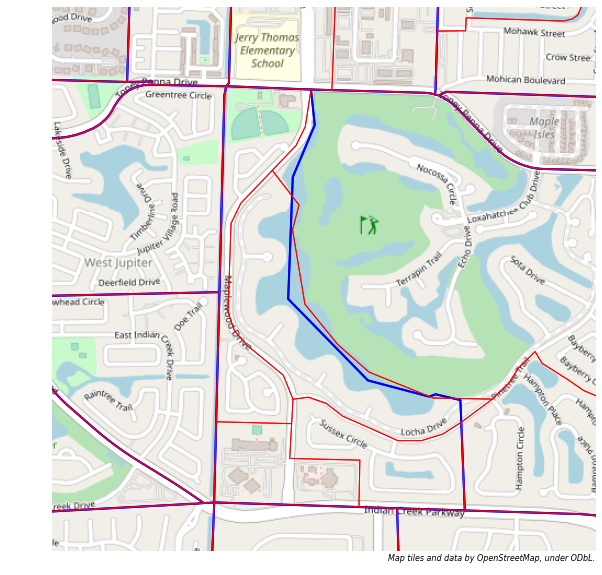
When the intersection of the two zone systems is computed, half a dozen extraneous small zones are generated along the lake that forms the western edge of the golf course, but these are not actually meaningful activity locations and are not relevant for transortation analysis.
The possible solutions to both problems are the same, given that we know that the “correct” join solution will have exactly one zone in the result for each MAZ.
Dropping Extra Pieces
One possible solution is to take the joined data we already have, and remove all the extra pieces of zones that were created, retaining only the largest main section of each MAZ. To do this, we can sort zones in the joined GeoDataFrame by area, and retain only the largest zone from each group of duplicated MAZ codes.
First, we’ll use the argsort method, to get the order of the joined zones, if ordered by area. Then we feed that into the iloc indexer to actually sort the rows as indicated. The argsort returns values in ascending order by default, so all the small slivers and bits of zones we want to discard will appear first.
[39]:
maz_taz = maz_taz.iloc[maz_taz.area.argsort()]
Then, we can drop duplicate MAZ values from the table, keeping only the last instance of each MAZ, which is the one we want. In theory, if the two zones systems are very poorly aligned, this process could drop the wrong part of the zones, although in almost all cases it will work fine.
[40]:
maz_taz = maz_taz.drop_duplicates('MAZ', keep='last')
[41]:
len(maz_taz)
[41]:
361
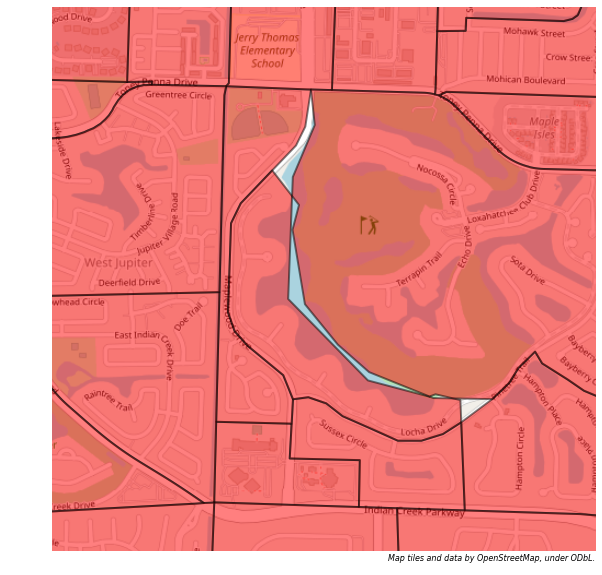
[42]:
ax = tt.mapping.make_basemap(xlim=(938500,945500), ylim=(937500,944500), zoom=15, tiles='OSM_A', epsg=2236, axis='off')
ax = maz_taz.plot(ax=ax, edgecolor='k', linewidth=2, facecolor='r', alpha=0.5 )
Joining on Centroids
An alternate solution is to join the TAZ and MAZ data in a entirely different manner. Rather than joining the two GeoDataFrames based on the area polygons in each, we can join based on the area polygons for TAZ’s and centroids for MAZ’s. To do this, we’ll use the sjoin method.
First, we’ll need a version of the MAZ GeoDataFrame that has only centroid points in the geometry column, instead of polygons. To create this, start by making a copy of the original data (assuming we want to save it for later).
[43]:
maz_points = maz_jupiter.copy()
Then we want to change the geometry to be points instead of polygons. (Both Point and Polygon are specific object types in the shapely package that is used by GeoPandas.) We could simply use the ‘centroid’ attribute of the geometry column to find new centroid for each zone, but in this data we already have X and Y values for a centroid, so we’ll prefer to use those. We can uses the apply method of DataFrames to create Point values, and assign those values into the geometry column.
[44]:
from shapely.geometry import Point
maz_points.geometry = maz_points.apply(lambda x: Point(x.POINT_X, x.POINT_Y), axis=1)
[45]:
sjoined = gpd.sjoin(maz_points, taz_jupiter, how='left', op='within')
[46]:
len(sjoined)
[46]:
361
[47]:
sjoined.head()
[47]:
| OBJECTID_left | MAZ | SHAPE_LENG | SHAPE_AREA | ACRES | POINT_X | POINT_Y | geometry | index_right | OBJECTID_right | ... | COUNTY | CENSUSTAZ | TAZ_BF | FIX | AREA | F_NETAREA | CBD | HM_ROOMS | Shape_Leng | Shape_Area | |
|---|---|---|---|---|---|---|---|---|---|---|---|---|---|---|---|---|---|---|---|---|---|
| 2388 | 2389 | 7736 | 10592.846522 | 4.442490e+06 | 102 | 936259 | 957308 | POINT (936259 957308) | 0 | 1 | ... | 1.0 | None | 0 | 0 | 4442490.0 | 0.8153 | 0 | 0 | 10592.846522 | 4.442490e+06 |
| 2389 | 2390 | 7737 | 17396.297932 | 1.568938e+07 | 360 | 940102 | 950911 | POINT (940102 950911) | 1 | 2 | ... | 1.0 | None | 0 | 0 | 15689400.0 | 0.8571 | 0 | 0 | 17396.297932 | 1.568938e+07 |
| 2390 | 2391 | 7738 | 18511.806088 | 1.405994e+07 | 323 | 937715 | 953796 | POINT (937715 953796) | 2 | 3 | ... | 1.0 | None | 0 | 0 | 17396100.0 | 0.8663 | 0 | 0 | 23585.421941 | 1.739613e+07 |
| 2391 | 2392 | 7739 | 7202.864864 | 1.303422e+06 | 30 | 953218 | 953704 | POINT (953218 953704) | 3 | 4 | ... | 1.0 | None | 0 | 0 | 1303420.0 | 0.8536 | 0 | 0 | 7202.864864 | 1.303422e+06 |
| 2392 | 2393 | 7740 | 24940.959492 | 3.147748e+07 | 723 | 931973 | 952018 | POINT (931973 952018) | 4 | 5 | ... | 1.0 | None | 0 | 0 | 31477500.0 | 0.8787 | 0 | 0 | 24940.959492 | 3.147748e+07 |
5 rows × 23 columns
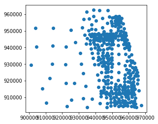
The resulting GeoDataFrame has the geometry from the left input, which in this case is just the centroid points.
[48]:
ax = sjoined.plot()
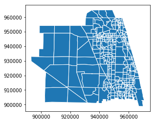
If we want to re-attach the polygon zones, we can do so easily if we didn’t overwrite the original MAZ data, because this joined data is in the same order as the original.
[49]:
sjoined.MAZ.equals(maz_jupiter.MAZ)
[49]:
True
[50]:
sjoined.geometry = maz_jupiter.geometry
[51]:
ax = sjoined.plot(edgecolor='w')
Creating a Crosswalk Dictionary from the Joined Data
We will sometimes be given a MAZ id but want to get the TAZ id instead. As this is a one-to-many mapping (every MAZ is in one and only one TAZ, but each TAZ can contain multiple MAZ’s), it is convenient to express this mapping as a Python dictionary. This can be done easily if the index of the GeoDataFrame is set to be the MAZ.
[52]:
sjoined.index=sjoined.MAZ
[53]:
maz_taz_crosswalk = dict(sjoined.TAZ_MPO)
Then, given a MAZ number we can access the TAZ simply like this:
[54]:
maz_number = 7755
taz_number = maz_taz_crosswalk[maz_number]