Using Selection by Geography

import transportation_tutorials as tt
import geopandas as gpd
import pandas as pd
import matplotlib.pyplot as plt
import osmnx as ox
from shapely.geometry import Polygon

Questions

Consider a study area that mostly covers Deerfield Beach in Florida. The study area can be defined by a polygon bounded by the following coordinates (given in epsg:4326):

Polygon([
    (-80.170862, 26.328588),
    (-80.170158, 26.273494),
    (-80.113007, 26.274882),
    (-80.104592, 26.293503),
    (-80.072967, 26.293790),
    (-80.070111, 26.329349)
])

1. Use OSMnx to download the boundaries for Deerfield Beach, and generate an image that compares the city to the indicated study area polygon. Are there any areas in the city of Deerfield Beach that are outside the designated studay area, and if so, is this concerning? (Hint: use the ``add_basemap`` function from the ``transportation_tutorials.mapping`` package to add context to your map.)
2. How many MAZs are there that are located completely inside the study area? Generate a static map of only these MAZ’s. (Hint: Please make sure to use appropriate Coordinate Reference Systems (CRS) in your analysis.)
3. How many MAZs are at least partially inside the study area? Generate a static map of these MAZ’s, including the full area of any MAZ that is at least partially contained in the study area.

Data

To answer the questions, use the following file:

maz = gpd.read_file(tt.data('SERPM8-MAZSHAPE'))

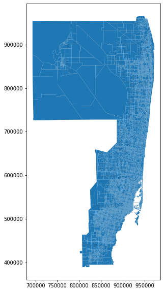
maz.plot(figsize = (10,10));

maz.head()

	OBJECTID	MAZ	SHAPE_LENG	SHAPE_AREA	ACRES	POINT_X	POINT_Y	geometry
0	1	5347	8589.393674	3.111034e+06	71	953130	724165	POLYGON ((953970.4660769962 723936.0810402408,...
1	2	5348	11974.067469	7.628753e+06	175	907018	634551	POLYGON ((908505.2801046632 635081.7738410756,...
2	3	5349	9446.131753	4.007041e+06	92	923725	707062	POLYGON ((922736.6374686621 708387.6918614879,...
3	4	5350	21773.153739	2.487397e+07	571	908988	713484	POLYGON ((908334.2374677472 715692.2628822401,...
4	5	5351	17882.701416	1.963139e+07	451	909221	717493	POLYGON ((911883.0187559947 719309.3261861578,...

Solution

First, we create a variable from the defined polygon for our study area. The coordinates are given in epsg:4326 format, which is the same as the coordinate system used by OpenStreetMaps, so we do not yet need to convert our data.

clipper_poly = Polygon([
    (-80.170862, 26.328588),
    (-80.170158, 26.273494),
    (-80.113007, 26.274882),
    (-80.104592, 26.293503),
    (-80.072967, 26.293790),
    (-80.070111, 26.329349)
])

Then, we can download the Deerfield Beach data from OpenStreetMap:

city = ox.gdf_from_place('Deerfield Beach, Florida, USA')

And plot them together:

ax = city.plot()
lines = ax.plot(*clipper_poly.exterior.xy, color = 'r')

The shape we received from OpenStreetMap does indeed have some area outside the study area polygon. To identify whether we should be concerned, it will be useful to have some context about what exactly is in that region. We can use the add_basemap function to attach some map tiles to our map that will give us the necessary context:

ax = city.plot(alpha=0.5)
lines = ax.plot(*clipper_poly.exterior.xy, color = 'r')
ax = tt.mapping.add_basemap(ax, zoom=13, epsg=4326)

Looks like that part of Deerfield Beach from OSM that’s not in our study area is out in the Atlantic Ocean. We’ve not going to be studying boaters today, so we can safely ignore this discrepancy.

To evaluate the MAZ’s relative to the study area, we’ll use the provided MAZ shapefile data. We can check the coordinate reference system used for this data:

maz.crs

{'init': 'epsg:2236'}

And we find that it is not the same as the other data available, which is in EPSG:4326. We can use GeoPandas to reformat the study area polygon to be in the same crs as the MAZ data like this:

clipper_gdf = gpd.GeoDataFrame(index=[0], crs={'init': 'epsg:4326'}, geometry=[clipper_poly]).to_crs(epsg=2236)
clipper_poly = clipper_gdf.geometry[0]

Or, we could change the MAZ data to match the crs of the study area:

maz_4326 = maz.to_crs(epsg = 4326)

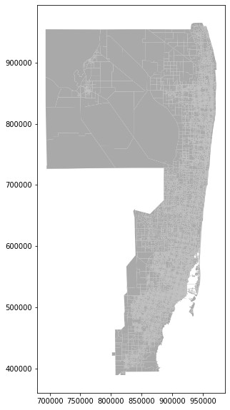
For this work, we’ll stick with the former, as EPSG:2236 is better suited to reduce distortion on map renders in Florida. We can plot the study area polygon over MAZs to see the location of study area within the region.

ax = maz.plot(figsize = (10,10), color = 'darkgrey')
clipper.plot(ax=ax);

---------------------------------------------------------------------------
NameError                                 Traceback (most recent call last)
<ipython-input-13-f37f778972d1> in <module>
      1 ax = maz.plot(figsize = (10,10), color = 'darkgrey')
----> 2 clipper.plot(ax=ax);

NameError: name 'clipper' is not defined

To render just the study area and the MAZs that fall completely inside the study area, we use .within() method as boolean mask for selection.

maz_within = maz[maz.within(clipper.geometry[0])]
ax = maz_within.plot(figsize = (10,10), color = 'grey', edgecolor = 'w')
clipper.plot(ax=ax, color='none', edgecolor = 'r');

Now, we can use maz_within dataframe to find our answer to the first question.

print('There are {} MAZs inside the study area.'.format(maz_within.shape[0]))

To instead include all the MAZ’s that touch the study area polygon, including those that are partially outside it, we can repeat the same code using intersects instead of within.

maz_intersects = maz[maz.intersects(clipper_poly)]
ax = maz_intersects.plot(
    figsize = (10,10),
    color = 'grey',
    edgecolor = 'w'
)
clipper.plot(ax=ax, color='none', edgecolor = 'r');

print('There are {} MAZs at least partially inside the study area.'.format(maz_intersects.shape[0]))